INTRODUCTION

Modern transportation is being transformed by autonomous cars, which provide safe, effective, and intelligent navigation. The Raspberry pi  AI, an effective and affordable single-board computer, is used in this research to demonstrate an autonomous path-following vehicle. The autonomous vehicle is made to follow predetermined routes while recognizing and avoiding obstacles in real-time. The Raspberry pi board AI-based system demonstrates a scalable and flexible solution for intelligent robotic applications by combining computer vision, control algorithms, and sensor integration. 

        1.1Raspberry pi : AN IDEAL PLATFORM: 

The second section explores the distinctive qualities of the Raspberry pi AI that make it a good platform for creating autonomous systems. We analyze its processing power, number of I/O ports, and Linux-based operating system, all of which make efficient integration with numerous sensors and actuators possible. 

        1.2 HARDWARE CONFIGURATION: 

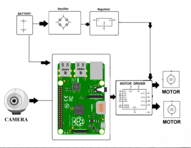
The hardware of the autonomous vehicle is described in the third part. This consists of a camera for computer vision tasks, an IMU for orientation estimation, DC motors with encoders for motion control, ultrasonic sensors for obstacle detection, and the Raspberry pi  AI functioning as the main processing unit. 

        1.3 SOFTWARE ARCHITECTURE: 

The software architecture of the autonomous vehicle is presented in Section 4. The Robot Operating System (ROS), which controls communication between various modules, is implemented on the Linux-based operating system that powers the Raspberry AI. We go through methods to integrate sensor drivers, computer vision libraries, control strategies, and reasoning for making decisions. 

        1.4 PATH FOLLOWING ALGORITHM: 

The path-following algorithm is described in more detail in the fifth section. Using sensor data, the automobile adjusts its speed and direction in order to maintain the desired trajectory. We go through how PID control or Model Predictive Control (MPC) is put into practice for accurate and fast path tracking.

        1.5 OBSTACLE IDENTIFICATION: 

We can determine the locations and dimensions of the observed obstacles and prevent collisions by employing methods like color-based detection, edge detection, contour detection, or template matching. The contour detection and clever edge detection algorithm are displayed in  a below Figure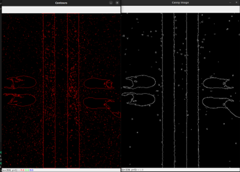

STEP 1 – Thresholding

Now the idea here is to get the path using either Color or Edge Detection. In our case we are using regular A4 White paper as path, therefore we can simply use the color detection to find the path. We will write the Thresholding function in the Utilities file.

def thresholding (img):   
   hsv = cv2.cvtColor(img,cv2.COLOR_BGR2HSV)
  lowerWhite = np.array([85, 0, 0])  
  upperWhite = np.array([179, 160, 255])    
 maskedWhite= cv2.inRange(hsv, lowerWhite, upperWhite)   
 return maskedWhite
Color Picker Script
import cv2
import numpy as np

frameWidth = 640
frameHeight = 480
cap = cv2.VideoCapture(1)
cap.set(3, frameWidth)
cap.set(4, frameHeight)
  def empty(a):
   pass
cv2.namedWindow("HSV")
cv2.resizeWindow("HSV", 640, 240)
cv2.createTrackbar("HUE Min", "HSV", 0, 179, empty)
cv2.createTrackbar("HUE Max", "HSV", 179, 179, empty)
cv2.createTrackbar("SAT Min", "HSV", 0, 255, empty)
cv2.createTrackbar("SAT Max", "HSV", 255, 255, empty)
cv2.createTrackbar("VALUE Min", "HSV", 0, 255, empty)
cv2.createTrackbar("VALUE Max", "HSV", 255, 255, empty)


cap = cv2.VideoCapture('vid1.mp4')
frameCounter = 0
  while True:
    frameCounter +=1    if cap.get(cv2.CAP_PROP_FRAME_COUNT) ==frameCounter:                                     cap.set(cv2.CAP_PROP_POS_FRAMES,0)
       frameCounter=0  
  _, img = cap.read()  
  imgHsv = cv2.cvtColor(img, cv2.COLOR_BGR2HSV)
     h_min = cv2.getTrackbarPos("HUE Min", "HSV")
    h_max = cv2.getTrackbarPos("HUE Max", "HSV")
   s_min = cv2.getTrackbarPos("SAT Min", "HSV")
    s_max = cv2.getTrackbarPos("SAT Max", "HSV")
   v_min = cv2.getTrackbarPos("VALUE Min", "HSV")
   v_max = cv2.getTrackbarPos("VALUE Max", "HSV")
   print(h_min)    lower = np.array([h_min, s_min, v_min])
   upper = np.array([h_max, s_max, v_max])
    mask = cv2.inRange(imgHsv, lower, upper)
   result = cv2.bitwise_and(img, img, mask=mask)
     mask = cv2.cvtColor(mask, cv2.COLOR_GRAY2BGR)
    hStack = np.hstack([img, mask, result])
   cv2.imshow('Horizontal Stacking', hStack)
   if cv2.waitKey(1) and 0xFF == ord('q'):
        break cap.release()
cv2.destroyAllWindows()

 STEP 2 –Warping

We don’t want to process the whole image because we just want to know the curve on the path right now and not a few seconds ahead. So we can simply crop our image, but this is not enough since we want to look at the road as if we were watching from the top . This is known as a bird eye view and it is important because it will allow us to easily find the curve. To warp the image we need to define the initial points. These points we can determine manually. So to make this process easier we could use track bars to experiment with different values. The idea is to get a rectangle shape when the road is straight.

We can create two functions for the trackbars. One that initializes the trackbars and the second that get the current value from them.
 

def nothing(a):
    pass

def initializeTrackbars(intialTracbarVals,wT=480, hT=240):
    cv2.namedWindow("Trackbars")
    cv2.resizeWindow("Trackbars", 360, 240)
   cv2.createTrackbar("Width Top", "Trackbars", intialTracbarVals[0],wT//2, nothing)
   cv2.createTrackbar("Height Top", "Trackbars", intialTracbarVals[1], hT, nothing)  
  cv2.createTrackbar("Width Bottom", "Trackbars", intialTracbarVals[2],wT//2, nothing)
   cv2.createTrackbar("Height Bottom", "Trackbars", intialTracbarVals[3], hT, nothing)
def valTrackbars(wT=480, hT=240):
    widthTop = cv2.getTrackbarPos("Width Top", "Trackbars")
    heightTop = cv2.getTrackbarPos("Height Top", "Trackbars")
    widthBottom = cv2.getTrackbarPos("Width Bottom", "Trackbars")
   heightBottom = cv2.getTrackbarPos("Height Bottom", "Trackbars")
    points = np.float32([(widthTop, heightTop), (wT-widthTop, heightTop),
                     (widthBottom , heightBottom ), (wT-widthBottom, heightBottom)])
   return points

Now we can call the initialize function at the start of the code and the valTrackbar in the while loop just before warping the image. Since both functions are written in the utlis file we will write ‘utlis.’ before calling them.

intialTracbarVals = [110,208,0,480]
utlis.initializeTrackbars(intialTracbarVals)
points = utlis.valTrackbars()

Now we will write our warping function that will allow us to get the bird eyes view using the four points that we just tuned.

def warpImg (img,points,w,h,inv=False):
    pts1 = np.float32(points)
    pts2 = np.float32([[0,0],[w,0],[0,h],[w,h]])   
 if inv:
        matrix = cv2.getPerspectiveTransform(pts2,pts1)
   else:
       matrix = cv2.getPerspectiveTransform(pts1,pts2)  
  imgWarp = cv2.warpPerspective(img,matrix,(w,h))  
  return imgWarp

Here we are getting the transformation matrix based on the input points and then warping the image using the ‘warpPrespective’ function. Since we will also need to apply inverse Warping later on, we will add this functionality to our function. To inverse, we just need the inverse matrix which we can find by switching the pts1 and pts2.

Now we call our function to get the warp perspective.

imgWarp = utlis.warpImg(imgThres, points, wT, hT)

Its a good idea to visualize our points to make the tuning process easier. So to display our points we can create a new function that loops through the points and draws them using the ‘circle’ function.

def drawPoints(img,points):  
  for x in range( 0,4):  
      cv2.circle(img,(int(points[x][0]),int(points[x][1])),15,(0,0,255),cv2.FILLED)   
 return img

Now we can call this function to draw the points.

	
imgWarpPoints = utlis.drawPoints(imgWarpPoints, points)

Histogram

Now comes the most important part, finding the curve in our path . To do this we will use the summation of pixels. But what is that? Given that our Warped image is now binary i.e it has either black or white pixels, we can sum the pixel values in the y direction. Lets look at this in more detail.

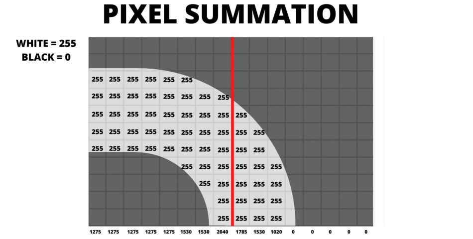
The picture above shows all the white pixels with 255 value and all the black with 0. Now if we sum the pixels in first column it yeilds 255+255+255+255+255 = 1275. We apply this method to each of the columns. In our original Image we have 480 pixels in the width. Therefore we will have 480 values. After summation we can look at how many values are above a certain threshold hold lets say 1000 on each side of the center red line. In the above example we have 8 columns on the left and 3 columns on the right. This tells us that the curve is towards left. This is the basic concept, though we will add a few more things to improve this and get consistent results. But if we look deeper into this we will face a problem. Lets have a look.

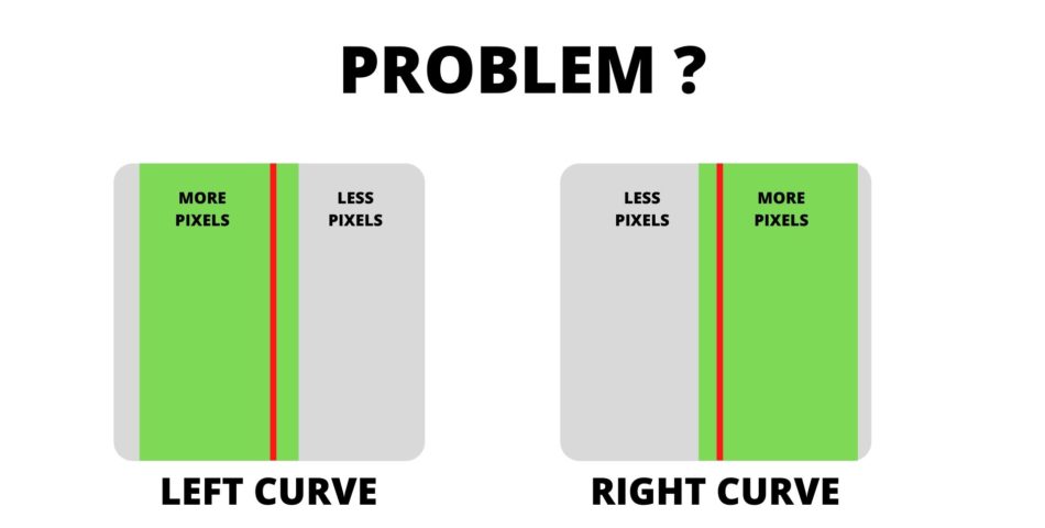
Here even though there is no curve since more pixels are present on one side the algorithm will output either left or right curve. So how can we fix this problem. The answer is simple we adjust the center line.

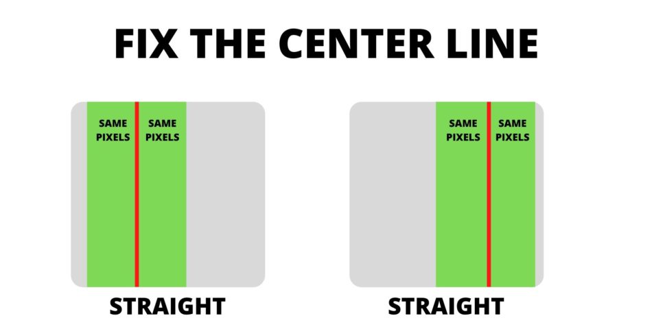
So now we have to find the center of the base which will give us the center line and then compare the pixels on both side.

Lucky for us both processes can be computed with the same function. By sumation of these pixels we are basically finding the histogram. Therefore we will call this function ‘getHistogram’. Lets assume we are doing the second step where we have to sum all the pixels and later we will come back to step one to find the center of the base.

Conclusion 

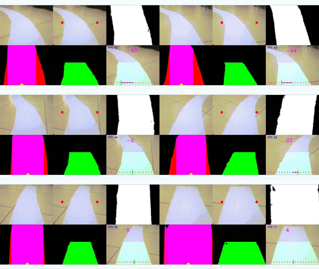
The conclusion of the project autonomous path following a car using Raspberry is a successful implementation. The Raspberry capabilities allow it to perform real-time processing and make real-time decisions while navigating the path.   

Looking ahead there are several promising directions in the research of autonomous path-following car using Raspberry. 

Autonomous path-following vehicles powered by Raspberry or other embedded systems have a bright future. We may anticipate a number of advances and opportunities in this subject as technology develops:

Advanced Machine Learning and AI: For vision, decision-making, and control, autonomous vehicles significantly rely on machine learning and artificial intelligence. Automobiles will be able to comprehend and navigate complicated and dynamic situations better in the future thanks to developments in AI algorithms, neural networks, and deep learning models. 

Improved Sensor Technology: Autonomous vehicles can sense their environment by using a variety of sensors, including LiDAR, radar, cameras, and ultrasonic sensors. Expect to see advancements in sensor technology, such as improved resolution, longer ranges, and lower costs, which will increase the capability and affordability of autonomous cars.

Robotics and Automation: The pi Car project can be used to investigate topics other than cars, such as robotics, automation, and industrial applications. By adding new hardware components, it can be improved in robotics and automation applications.